Univariate Data with the Normal Inverse Chi-Square Distribution
One of the simplest examples of data is univariate data
Let’s consider a timeseries example:
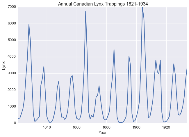
The Annual Canadian Lynx Trappings Dataset as described by Campbel and Walker 1977 contains the number of Lynx trapped near the McKenzie River in the Northwest Territories in Canada between 1821 and 1934.
import pandas as pd
import numpy as np
import seaborn as sns
import matplotlib.pyplot as plt
%matplotlib inline
sns.set_context('talk')
sns.set_style('darkgrid')
lynx = pd.read_csv('https://vincentarelbundock.github.io/Rdatasets/csv/datasets/lynx.csv',
                   index_col=0)
lynx = lynx.set_index('time')
lynx.head()
| lynx | |
|---|---|
| time | |
| 1821 | 269 |
| 1822 | 321 |
| 1823 | 585 |
| 1824 | 871 |
| 1825 | 1475 |
lynx.plot(legend=False)
plt.xlabel('Year')
plt.title('Annual Canadian Lynx Trappings 1821-1934')
plt.ylabel('Lynx')
<matplotlib.text.Text at 0x1129d0090>
Let’s plot the kernel density estimate of annual lynx trapping
sns.kdeplot(lynx['lynx'])
plt.title('Kernel Density Estimate of Annual Lynx Trapping')
plt.ylabel('Probability')
plt.xlabel('Number of Lynx')
<matplotlib.text.Text at 0x1129d0410>
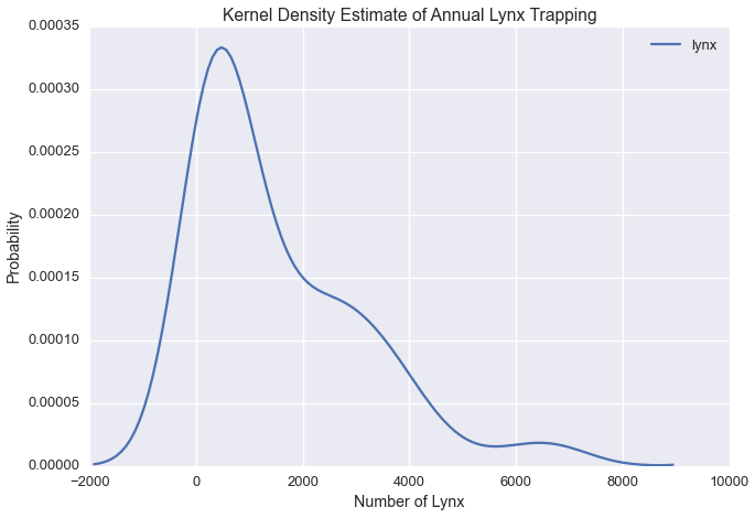
Our plot suggests there could be three modes in the Lynx data.
In modeling this timeseries, we could assume that the number of lynx trapped in a given year is falls into one of \(k\) states, which are normally distributed with some unknown mean \(\mu_i\) and variance \(\sigma^2_i\) for each state
In the case of our Lynx data
Now let’s consider demographics data from the Titanic Dataset
The Titanic Dataset contains information about passengers of the Titanic.
ti = sns.load_dataset('titanic')
ti.head()
| survived | pclass | sex | age | sibsp | parch | fare | embarked | class | who | adult_male | deck | embark_town | alive | alone | |
|---|---|---|---|---|---|---|---|---|---|---|---|---|---|---|---|
| 0 | 0 | 3 | male | 22 | 1 | 0 | 7.2500 | S | Third | man | True | NaN | Southampton | no | False |
| 1 | 1 | 1 | female | 38 | 1 | 0 | 71.2833 | C | First | woman | False | C | Cherbourg | yes | False |
| 2 | 1 | 3 | female | 26 | 0 | 0 | 7.9250 | S | Third | woman | False | NaN | Southampton | yes | True |
| 3 | 1 | 1 | female | 35 | 1 | 0 | 53.1000 | S | First | woman | False | C | Southampton | yes | False |
| 4 | 0 | 3 | male | 35 | 0 | 0 | 8.0500 | S | Third | man | True | NaN | Southampton | no | True |
Passenger age and fare are both real valued. Are they related? Let’s examine the correlation matrix
ti[['age','fare']].dropna().corr()
| age | fare | |
|---|---|---|
| age | 1.000000 | 0.096067 |
| fare | 0.096067 | 1.000000 |
Since the correlation is between the two variables is zero, we can model these two real valued columns independently.
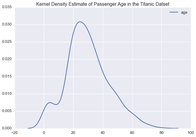
Let’s plot the kernel density estimate of each variable
sns.kdeplot(ti['age'])
plt.title('Kernel Density Estimate of Passenger Age in the Titanic Datset')
<matplotlib.text.Text at 0x117426c50>
sns.kdeplot(ti['fare'])
plt.title('Kernel Density Estimate of Passenger Fare in the Titanic Datset')
<matplotlib.text.Text at 0x117475310>
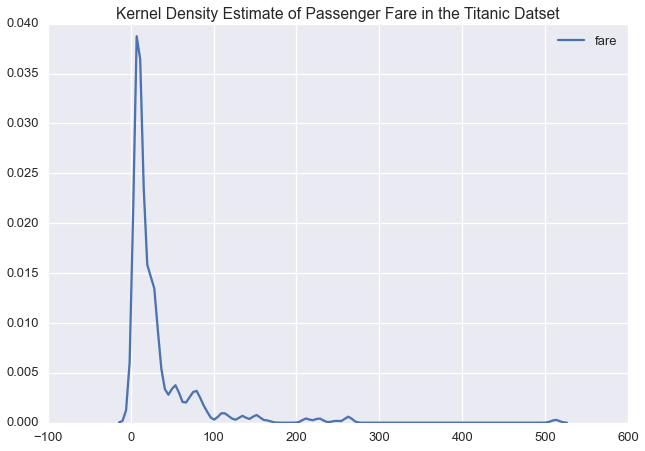
Given the long tail in the fare price, we might want to model this variable on a log scale:
ti['logfare'] = np.log(ti['fare'])
ti[['age','logfare']].dropna().corr()
| age | logfare | |
|---|---|---|
| age | 1.000000 | 0.135352 |
| logfare | 0.135352 | 1.000000 |
Again, logfare and age have near zero correlation, so we can
again model these two variables independently
Let’s see what a kernel density estimate of log fare would look like
sns.kdeplot(ti['logfare'])
plt.title('Kernel Density Estimate of Log Passenger Fare in the Titanic Datset')
<matplotlib.text.Text at 0x1175a5110>
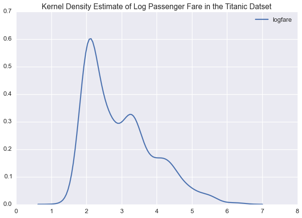
In logspace, passenger fare is multimodal, suggesting that we could model this variable with a normal distirbution
If we were to model the passenger list using our Mixture Model, we would
have separate likelihoods for logfare and age
Often, real value data is assumed to be normally distributed.
To learn the latent variables, \(\mu_i\) \(\sigma^2_i\), we would use a normal inverse-chi-square likelihood
The normal inverse-chi-square likelihood is the conjugate univariate normal likelihood in data microscopes. We also have normal likelihood, the normal inverse-wishart likelihood, optimized for multivariate datasets.
It is important to model univariate normal data with this likelihood as it acheives superior performance on univariate data.
In both these examples, we found variables that were amenable to being modeled as univariate normal:
- Univariate datasets
- Datasets containing real valued variables with near zero correlation
To import our univariate normal inverse-chi-squared likelihood, call:
from microscopes.models import nich as normal_inverse_chisquared