Digit recognition with the MNIST dataset¶

Let’s set up our environment

%matplotlib inline
import matplotlib.pylab as plt
import numpy as np
import numpy.ma as ma
import time
import math
import seaborn as sns

from PIL import Image, ImageOps
from sklearn.datasets import fetch_mldata

Now let’s get our functions from datamicroscopes

from microscopes.models import bb as beta_bernoulli
from microscopes.mixture.definition import model_definition
from microscopes.common.rng import rng
from microscopes.common.recarray.dataview import numpy_dataview
from microscopes.mixture import model, runner, query
from microscopes.kernels import parallel

Let’s focus on classifying 2’s and 3’s

mnist_dataset = fetch_mldata('MNIST original')
Y_2 = mnist_dataset['data'][np.where(mnist_dataset['target'] == 2.)[0]]
Y_3 = mnist_dataset['data'][np.where(mnist_dataset['target'] == 3.)[0]]
print 'number of twos:', Y_2.shape[0]
print 'number of threes:', Y_3.shape[0]

number of twos: 6990
number of threes: 7141

print 'number of dimensions: %d' % len(Y_2.shape)

number of dimensions: 2

Our data is 2 dimensional, which means each observation is a vector.

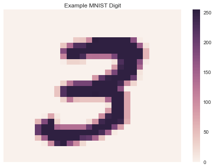
We can reformat our data to show the digits as images

_, D = Y_3.shape
W = int(math.sqrt(D))
assert W * W == D
sns.heatmap(np.reshape(Y_3[0], (W, W)), linewidth=0, xticklabels=False, yticklabels=False)
plt.title('Example MNIST Digit')

<matplotlib.text.Text at 0x119273fd0>

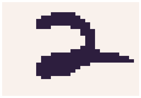
For simplicity, we’ll convert these grayscale images into binary images

To pass our data into datamicroscopes, we’ll also munge the data into recarray format

Y = np.vstack([Y_2, Y_3])
Y = np.array([tuple(y) for y in np.random.permutation(Y)], dtype=[('', bool)]*D)

Let’s look at an example image

sns.heatmap(np.reshape([i for i in Y[0]], (W,W)), linewidth=0, xticklabels=False, yticklabels=False, cbar=False)

<matplotlib.axes._subplots.AxesSubplot at 0x1134c8cd0>

Now, we can initialize our model. To do so, we must:

Specify the number of chains
Import the data
Define the model
Initialize the model
Initialize the samplers, aka runners

For this classification task, we’ll use a Dirichlet Process Mixture Model

Since we converted the data into binary vectors for each pixel, we’ll define our likelihood of the model as a beta-bernouli. In this case, the likelihood is the probability that each of the \(D\) pixels in the image is True or False. Note, these pixel assignments are assumed to be independent.

\[\forall\hspace{2mm} d \in [0,1,..,D],\hspace{2mm} k \in [0,..,K], \hspace{2mm} P(pixel_d = True|cluster=k) \sim BetaBernoulli(\alpha_k,\beta_k)\]

\[\forall \hspace{2mm} d\neq c \hspace{2mm} P(pixel_d = True|cluster=k) \perp P(pixel_c = True|cluster=k)\hspace{2mm}\]

Recall that since we’re using a Dirichlet Process Mixture Model, \(K\) is also latent variable which we learn at these same time as the each cluster’s parameters

nchains = 5
view = numpy_dataview(Y)
defn = model_definition(Y.shape[0], [beta_bernoulli]*D)
prng = rng()
kc = runner.default_kernel_config(defn)
latents = [model.initialize(defn, view, prng) for _ in xrange(nchains)]
runners = [runner.runner(defn, view, latent, kc) for latent in latents]
r = parallel.runner(runners)
print '%d betabernouli likelihoods: one for each pixel' % len(defn.models())

784 betabernouli likelihoods: one for each pixel

Now let’s run each chain in parallel for 5 iterations

start = time.time()
iters = 5
r.run(r=prng, niters=iters)
print "mcmc took", (time.time() - start)/60., "minutes"

mcmc took 156.391473516 minutes
mcmc took 156.391473516 minutes

To save our results, we can get the latest assignment of each observation and pickle the output

infers = r.get_latents()

# save to disk
import pickle
with open("mnist-predictions-infers.pickle", 'w') as fp:
    pickle.dump(infers, fp)

import pickle
infers = pickle.load(open("mnist-predictions-infers.pickle"))

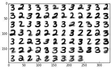
With our saved results, we can plot our learned clusters

def plot_clusters(s, scalebysize=False):
    hps = [s.get_feature_hp(i) for i in xrange(D)]
    def prior_prob(hp):
        return hp['alpha'] / (hp['alpha'] + hp['beta'])
    def data_for_group(gid):
        suffstats = [s.get_suffstats(gid, i) for i in xrange(D)]
        def prob(hp, ss):
            top = hp['alpha'] + ss['heads']
            bot = top + hp['beta'] + ss['tails']
            return top / bot
        probs = [prob(hp, ss) for hp, ss in zip(hps, suffstats)]
        return np.array(probs)
    def scale(d, weight):
        im = d.reshape((W, W))
        newW = max(int(weight * W), 1)
        im = Image.fromarray(im)
        im = im.resize((newW, newW))
        im = ImageOps.expand(im, border=(W - newW) / 2)
        im = np.array(im)
        a, b = im.shape
        if a < W:
            im = np.append(im, np.zeros(b)[np.newaxis,:], axis=0)
        elif a > W:
            im = im[:W,:]
        if b < W:
            im = np.append(im, np.zeros(W)[:,np.newaxis], axis=1)
        elif b > W:
            im = im[:,:W]
        return im.flatten()
    def groupsbysize(s):
        counts = [(gid, s.groupsize(gid)) for gid in s.groups()]
        counts = sorted(counts, key=lambda x: x[1], reverse=True)
        return counts
    data = [(data_for_group(g), cnt) for g, cnt in groupsbysize(s)]
    largest = max(cnt for _, cnt in data)
    data = [scale(d, cnt/float(largest))
            if scalebysize else d for d, cnt in data]
    digits_per_row = 12
    rem = len(data) % digits_per_row
    if rem:
        fill = digits_per_row - rem
        for _ in xrange(fill):
            data.append(np.zeros(D))
    rows = len(data) / digits_per_row
    data = np.vstack([
        np.hstack([d.reshape((W, W)) for d in data[i:i+digits_per_row]])
        for i in xrange(0, len(data), digits_per_row)])
    plt.imshow(data, cmap=plt.cm.binary, interpolation='nearest')
    plt.show()

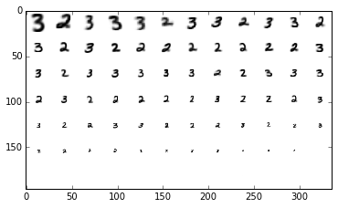
Let’s show all groups (also by size) for the first set of assignments

plt.hold(True)
plot_clusters(infers[0])
plot_clusters(infers[0], scalebysize=True)

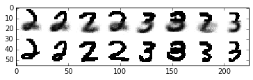
Now, let’s used our learned clusters to make predictions when presented with only the top half of the digit image

present = D/2
absent = D-present
queries = [tuple(Y_2[i]) for i in np.random.permutation(Y_2.shape[0])[:4]] + \
          [tuple(Y_3[i]) for i in np.random.permutation(Y_3.shape[0])[:4]]

queries_masked = ma.masked_array(
    np.array(queries, dtype=[('',bool)]*D),
    mask=[(False,)*present + (True,)*absent])

statistics = query.posterior_predictive_statistic(queries_masked, infers, prng, samples_per_chain=10, merge='avg')

data0 = np.hstack([np.array(list(s)).reshape((W,W)) for s in statistics])
data1 = np.hstack([np.clip(np.array(q, dtype=np.float), 0., 1.).reshape((W, W)) for q in queries])
data = np.vstack([data0, data1])
plt.imshow(data, cmap=plt.cm.binary, interpolation='nearest')

<matplotlib.image.AxesImage at 0x1256f1890>

<matplotlib.image.AxesImage at 0x1256f1890>