Categorical Data and the Dirichlet Discrete Distribution¶

Let’s consider some examples of data with categorical variables

import pandas as pd
import seaborn as sns
import numpy as np
import matplotlib.pyplot as plt
%matplotlib inline
sns.set_context('talk')
sns.set_style('darkgrid')

First, the passenger list of the Titanic

titanic = sns.load_dataset("titanic")

titanic.head(n=10)

	survived	pclass	sex	age	sibsp	parch	fare	embarked	class	who	adult_male	deck	embark_town	alive	alone
0	0	3	male	22	1	0	7.2500	S	Third	man	True	NaN	Southampton	no	False
1	1	1	female	38	1	0	71.2833	C	First	woman	False	C	Cherbourg	yes	False
2	1	3	female	26	0	0	7.9250	S	Third	woman	False	NaN	Southampton	yes	True
3	1	1	female	35	1	0	53.1000	S	First	woman	False	C	Southampton	yes	False
4	0	3	male	35	0	0	8.0500	S	Third	man	True	NaN	Southampton	no	True
5	0	3	male	NaN	0	0	8.4583	Q	Third	man	True	NaN	Queenstown	no	True
6	0	1	male	54	0	0	51.8625	S	First	man	True	E	Southampton	no	True
7	0	3	male	2	3	1	21.0750	S	Third	child	False	NaN	Southampton	no	False
8	1	3	female	27	0	2	11.1333	S	Third	woman	False	NaN	Southampton	yes	False
9	1	2	female	14	1	0	30.0708	C	Second	child	False	NaN	Cherbourg	yes	False

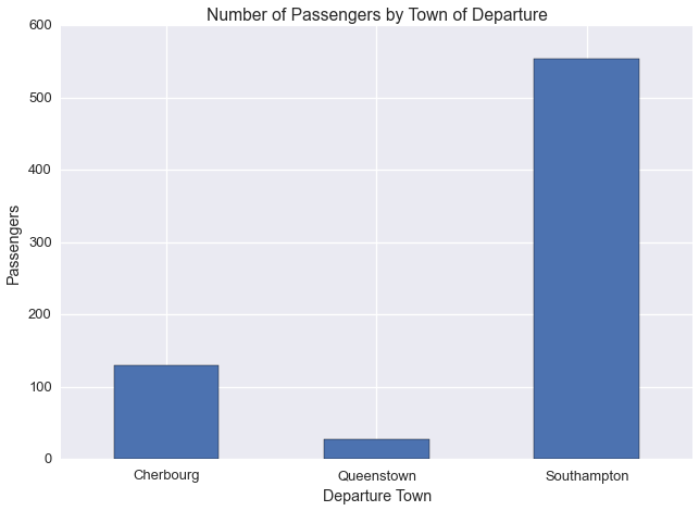
One of the categorical variables in this dataset is embark_town

Let’s plot the number of passengers departing from each town

ax = titanic.groupby(['embark_town'])['age'].count().plot(kind='bar')
plt.xticks(rotation=0)
plt.xlabel('Departure Town')
plt.ylabel('Passengers')
plt.title('Number of Passengers by Town of Departure')

<matplotlib.text.Text at 0x1029b9a10>

Let’s look at another example: the cars93 dataset

cars = pd.read_csv('https://vincentarelbundock.github.io/Rdatasets/csv/MASS/Cars93.csv', index_col=0)

cars.head()

	Manufacturer	Model	Type	Min.Price	Price	Max.Price	MPG.city	MPG.highway	AirBags	DriveTrain	...	Passengers	Length	Wheelbase	Width	Turn.circle	Rear.seat.room	Luggage.room	Weight	Origin	Make
1	Acura	Integra	Small	12.9	15.9	18.8	25	31	None	Front	...	5	177	102	68	37	26.5	11	2705	non-USA	Acura Integra
2	Acura	Legend	Midsize	29.2	33.9	38.7	18	25	Driver & Passenger	Front	...	5	195	115	71	38	30.0	15	3560	non-USA	Acura Legend
3	Audi	90	Compact	25.9	29.1	32.3	20	26	Driver only	Front	...	5	180	102	67	37	28.0	14	3375	non-USA	Audi 90
4	Audi	100	Midsize	30.8	37.7	44.6	19	26	Driver & Passenger	Front	...	6	193	106	70	37	31.0	17	3405	non-USA	Audi 100
5	BMW	535i	Midsize	23.7	30.0	36.2	22	30	Driver only	Rear	...	4	186	109	69	39	27.0	13	3640	non-USA	BMW 535i

5 rows × 27 columns

cars.ix[1]

Manufacturer                  Acura
Model                       Integra
Type                          Small
Min.Price                      12.9
Price                          15.9
Max.Price                      18.8
MPG.city                         25
MPG.highway                      31
AirBags                        None
DriveTrain                    Front
Cylinders                         4
EngineSize                      1.8
Horsepower                      140
RPM                            6300
Rev.per.mile                   2890
Man.trans.avail                 Yes
Fuel.tank.capacity             13.2
Passengers                        5
Length                          177
Wheelbase                       102
Width                            68
Turn.circle                      37
Rear.seat.room                 26.5
Luggage.room                     11
Weight                         2705
Origin                      non-USA
Make                  Acura Integra
Name: 1, dtype: object

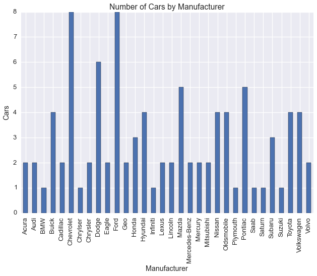
This dataset has multiple categorical variables

Based on the description of the cars93 datatset, we’ll consider Manufacturer, and DriveTrain to be categorical variables

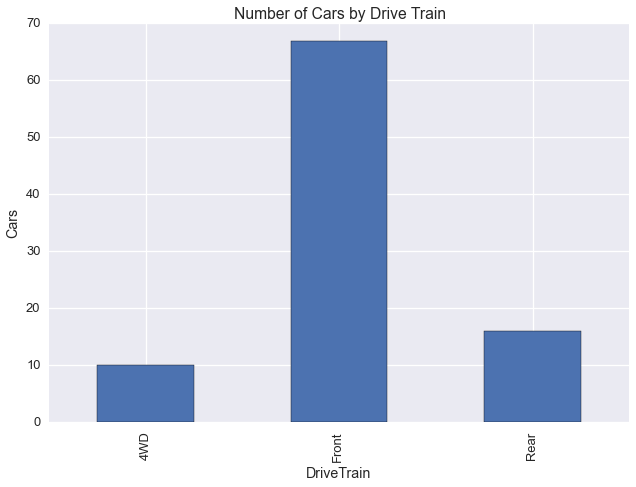
Let’s plot Manufacturer and DriveTrain

cars.groupby('Manufacturer')['Model'].count().plot(kind='bar')
plt.ylabel('Cars')
plt.title('Number of Cars by Manufacturer')

<matplotlib.text.Text at 0x114d9e6d0>

cars.groupby('DriveTrain')['Model'].count().plot(kind='bar')
plt.ylabel('Cars')
plt.title('Number of Cars by Drive Train')

<matplotlib.text.Text at 0x117554e50>

If our categorical data has labels, we need to convert them to integer id’s

def col_2_ids(df, col):
    ids = df[col].drop_duplicates().sort(inplace=False).reset_index(drop=True)
    ids.index.name = '%s_ids' % col
    ids = ids.reset_index()
    df = pd.merge(df, ids, how='left')
    del df[col]
    return df

cat_columns = ['Manufacturer', 'DriveTrain']

for c in cat_columns:
    print c
    cars = col_2_ids(cars, c)

Manufacturer
DriveTrain

cars[['%s_ids' % c for c in cat_columns]].head()

	Manufacturer_ids	DriveTrain_ids
0	0	1
1	0	1
2	1	1
3	1	1
4	2	2

Just as we model binary data with the beta Bernoulli distribution, we can model categorical data with the Dirichlet discrete distribution

The beta Bernoulli distribution allows us to learn the underlying probability, \(\theta\), of the binary random variable, \(x\)

\[P(x=1) =\theta\]

\[P(x=0) = 1-\theta\]

The Dirichlet discrete distribution extends the beta Bernoulli distribution to the case in which \(x\) can assume more than two states

\[\forall i \in [0,1,...n] \hspace{2mm} P(x = i) = \theta_i\]

\[\sum_{i=0}^n \theta_i = 1\]

Again, the Dirichlet distribution takes advantage of the fact that the Dirichlet distribution and the discrete distribution are conjugate. Note that the discrete distriution is sometimes called the categorical distribution or the multinomial distribution.

To import the Dirichlet discrete distribution call

from microscopes.models import dd as dirichlet_discrete

Then given the specific model we’d want we’d import

from microscopes.model_name.definition import model_definition

from microscopes.irm.definition import model_definition as irm_definition
from microscopes.mixture.definition import model_definition as mm_definition

See Defining Your Model to learn more about model definitions