Learning Topics in The Daily Kos with the Hierarchical Dirichlet Process
The Hierarchical Dirichlet Process (HDP) is typically used for topic modeling when the number of topics is unknown
Let’s explore the topics of the political blog, The Daily Kos using data from the UCI Machine Learning Repository.
import itertools
import pyLDAvis
import pandas as pd
import re
import simplejson
import seaborn as sns

from microscopes.common.rng import rng
from microscopes.lda.definition import model_definition
from microscopes.lda.model import initialize
from microscopes.lda import model, runner
from random import shuffle
import matplotlib.pyplot as plt

sns.set_style('darkgrid')
sns.set_context('talk')

%matplotlib inline
First, let’s grab the data from UCI:
!curl http://archive.ics.uci.edu/ml/machine-learning-databases/bag-of-words/docword.kos.txt.gz | gunzip > docword.kos.txt
!head docword.kos.txt
  % Total    % Received % Xferd  Average Speed   Time    Time     Time  Current
                                 Dload  Upload   Total   Spent    Left  Speed
100 1029k  100 1029k    0     0   129k      0  0:00:07  0:00:07 --:--:--  243k
3430
6906
353160
1 61 2
1 76 1
1 89 1
1 211 1
1 296 1
1 335 1
1 404 1
!curl http://archive.ics.uci.edu/ml/machine-learning-databases/bag-of-words/vocab.kos.txt > vocab.kos.txt
!head vocab.kos.txt
  % Total    % Received % Xferd  Average Speed   Time    Time     Time  Current
                                 Dload  Upload   Total   Spent    Left  Speed
100 55467  100 55467    0     0   163k      0 --:--:-- --:--:-- --:--:--  163k
aarp
abandon
abandoned
abandoning
abb
abc
abcs
abdullah
ability
aboard
The format of the docword.os.txt file is 3 header lines, followed by
NNZ triples:
---
D
W
NNZ
docID wordID count
docID wordID count
docID wordID count
docID wordID count
...
docID wordID count
docID wordID count
docID wordID count
---
We’ll process the data into a list of lists of words ready to be fed into our algorithm:
def parse_bag_of_words_file(docword, vocab):
    with open(vocab, "r") as f:
        kos_vocab = [word.strip() for word in f.readlines()]
        id_to_word = {i: word for i, word in enumerate(kos_vocab)}

    with open(docword, "r") as f:
        raw = [map(int, _.strip().split()) for _ in f.readlines()][3:]

    docs = []
    for _, grp in itertools.groupby(raw, lambda x: x[0]):
        doc = []
        for _, word_id, word_cnt in grp:
            doc += word_cnt * [id_to_word[word_id-1]]
        docs.append(doc)
    return docs, id_to_word
docs, id_to_word = parse_bag_of_words_file("docword.kos.txt", "vocab.kos.txt")
vocab_size = len(set(word for doc in docs for word in doc))
We must define our model before we intialize it. In this case, we need the number of docs and the number of words.
From there, we can initialize our model and set the hyperparameters
defn = model_definition(len(docs), vocab_size)
prng = rng()
kos_state = initialize(defn, docs, prng,
                        vocab_hp=1,
                        dish_hps={"alpha": 1, "gamma": 1})
r = runner.runner(defn, docs, kos_state)

print "number of docs:", defn.n, "vocabulary size:", defn.v
number of docs: 3430 vocabulary size: 6906
Given the size of the dataset, it’ll take some time to run.
We’ll run our model for 1000 iterations and save our results every 25 iterations.
%%time
step_size = 50
steps = 500 / step_size

print "randomly initialized model:", "perplexity:", kos_state.perplexity(), "num topics:", kos_state.ntopics()
for s in range(steps):
    r.run(prng, step_size)
    print "iteration:", (s + 1) * step_size, "perplexity:", kos_state.perplexity(), "num topics:", kos_state.ntopics()
randomly initialized model: perplexity: 6908.4715103 num topics: 9
iteration: 50 perplexity: 1590.22974737 num topics: 12
iteration: 100 perplexity: 1584.21787143 num topics: 13
iteration: 150 perplexity: 1578.62064887 num topics: 14
iteration: 200 perplexity: 1576.42299865 num topics: 15
iteration: 250 perplexity: 1575.98953602 num topics: 11
iteration: 300 perplexity: 1575.71624243 num topics: 13
iteration: 350 perplexity: 1575.37703244 num topics: 12
iteration: 400 perplexity: 1575.47578721 num topics: 13
iteration: 450 perplexity: 1575.69188913 num topics: 12
iteration: 500 perplexity: 1575.02874469 num topics: 14
CPU times: user 47min 46s, sys: 9.39 s, total: 47min 55s
Wall time: 53min 11s
pyLDAvis is a Python implementation of the LDAvis tool created by Carson Sievert.
LDAvis is designed to help users interpret the topics in a topic model that has been fit to a corpus of text data. The package extracts information from a fitted LDA topic model to inform an interactive web-based visualization.
prepared = pyLDAvis.prepare(**kos_state.pyldavis_data())
pyLDAvis.display(prepared)
LDA state objects are fully serializable with Pickle and cPickle.
import cPickle as pickle

with open('kos_state.pkl','wb') as f:
    pickle.dump(kos_state, f)

with open('kos_state.pkl','rb') as f:
    new_state = pickle.load(f)
kos_state.assignments() == new_state.assignments()
True
kos_state.dish_assignments() == new_state.dish_assignments()
True
kos_state.table_assignments() == new_state.table_assignments()
True
kos_state = new_state
We can generate term relevances (as defined by Sievert and Shirley 2014) for each topic.
relevance = new_state.term_relevance_by_topic()
Here are the ten most relevant words for each topic:
for topics in relevance:
    words = [word for word, _ in topics[:10]]
    print ' '.join(words)
dean edwards clark gephardt iowa primary lieberman democratic deans kerry
iraq war iraqi military troops soldiers saddam baghdad forces american
cheney guard bush mccain boat swift john kerry service president
senate race elections seat district republican house money gop carson
court delay marriage law ballot gay amendment rights ethics committee
kerry bush percent voters poll general polling polls results florida
people media party bloggers political time america politics internet message
november account electoral governor sunzoo contact faq password login dkosopedia
administration bush tax jobs commission health billion budget white cuts
ethic weber ndp exemplary bloc passion acts identifying realities responsibility
williams orleans freeper ditka excerpt picks anxiety edit trade edited
science scientists space environmental cell reagan emissions species cells researchers
zimbabwe blessed kingdom heaven interpretation anchor christ cargo clip owners
smallest demonstration located unusual zahn predebate auxiliary endangered merit googlebomb
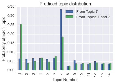
We can also predict how the topics with be distributed within an arbitrary document.
Let’s create a document from the 100 most relevant words in the 7th topic.
doc7 = [word for word, _ in relevance[6][:100]]
shuffle(doc7)
doc_text = [word for word in doc7]
print ' '.join(doc_text)
local reading party channel radio guys america dnc school ive sense hour movie times conservative ndn tnr talking coverage political heard lot air tom liberal moment discussion youre campaign learn wont bloggers heres traffic thought live speech media network isnt makes means boston weve organizations kind community blogging schaller jul readers convention night love life write news family find left read years real piece guest side event politics internet youll blogs michael long line ads dlc blog audience black stuff flag article country message journalists book blogosphere time tonight put ill email film fun people online matter blades theyre web
predictions = pd.DataFrame()
predictions['From Topic 7'] = pd.Series(kos_state.predict(doc, rng())[0])
The prediction is that this document is mostly generated by topic 7.
Similarly, if we create a document from words from the 1st and 7th topic, our prediction is that the document is generated mostly by those topics.
doc17 = [word for word, _ in relevance[0][:100]] + [word for word, _ in relevance[6][:100]]
shuffle(doc17)
predictions['From Topics 1 and 7']= pd.Series(kos_state.predict(doc17, r)[0])
predictions.plot(kind='bar')
plt.title('Prediced topic distribution')
plt.xticks(pred.index, ['%d' % (d+1) for d in xrange(len(pred.index))])
plt.xlabel('Topic Number')
plt.ylabel('Probability of Each Topic')
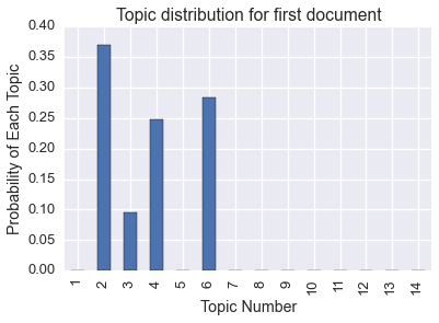
Of course, we can also get the topic distribution for each document (commonly called \(\Theta\)).
pd.Series(kos_state.topic_distribution_by_document()[0]).plot(kind='bar').set_title('Topic distribution for first document')
plt.xticks(pred.index, ['%d' % (d+1) for d in xrange(len(pred.index))])
plt.xlabel('Topic Number')
plt.ylabel('Probability of Each Topic')
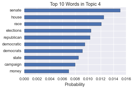
We can also get the raw word distribution for each topic (commonly called \(\Phi\)). This is related to the word relevance. Here are the most common words in one of the topics.
pd.Series(kos_state.word_distribution_by_topic()[3]).sort(inplace=False).tail(10).plot(kind='barh')
plt.title('Top 10 Words in Topic 4')
plt.xlabel('Probability')
To use our HDP, install our libary in conda:
$ conda install microscopes-lda