Datatypes and Bayesian Nonparametric Models
To understand data, we often categorize data as falling under a specific type of datatype. Understanding our underlying dataype gives structure to the problem of modeling the data.
Datamicroscopes provides tools to understand 4 particular datatypes:
- Real valued data
- Social network data
- Timeseries data
- Text data
import numpy as np
import pandas as pd
import itertools as it
import seaborn as sns
import scipy.io
import cPickle as pickle
%matplotlib inline
import pylab as plt
sns.set_style('darkgrid')
sns.set_context('talk')
The two most common datatypes are real valued data and discrete data
For example, let’s take the iris dataset
iris = sns.load_dataset('iris')
iris.head()
| sepal_length | sepal_width | petal_length | petal_width | species | |
|---|---|---|---|---|---|
| 0 | 5.1 | 3.5 | 1.4 | 0.2 | setosa |
| 1 | 4.9 | 3.0 | 1.4 | 0.2 | setosa |
| 2 | 4.7 | 3.2 | 1.3 | 0.2 | setosa |
| 3 | 4.6 | 3.1 | 1.5 | 0.2 | setosa |
| 4 | 5.0 | 3.6 | 1.4 | 0.2 | setosa |
In this case, species is a discrete variable and the other variables
are real valued
By understanding the form of the data, we can find a model that represents its underlying structure
In the case of the iris dataset, plotting the data shows that
indiviudal species exhibit a typical range of measurements
irisplot = sns.pairplot(iris, hue="species", palette='Set2', diag_kind="hist", size=2.5)
irisplot.fig.suptitle('Scatter Plots and KDE of Iris Data by Species', fontsize = 18)
irisplot.fig.subplots_adjust(top=.9)
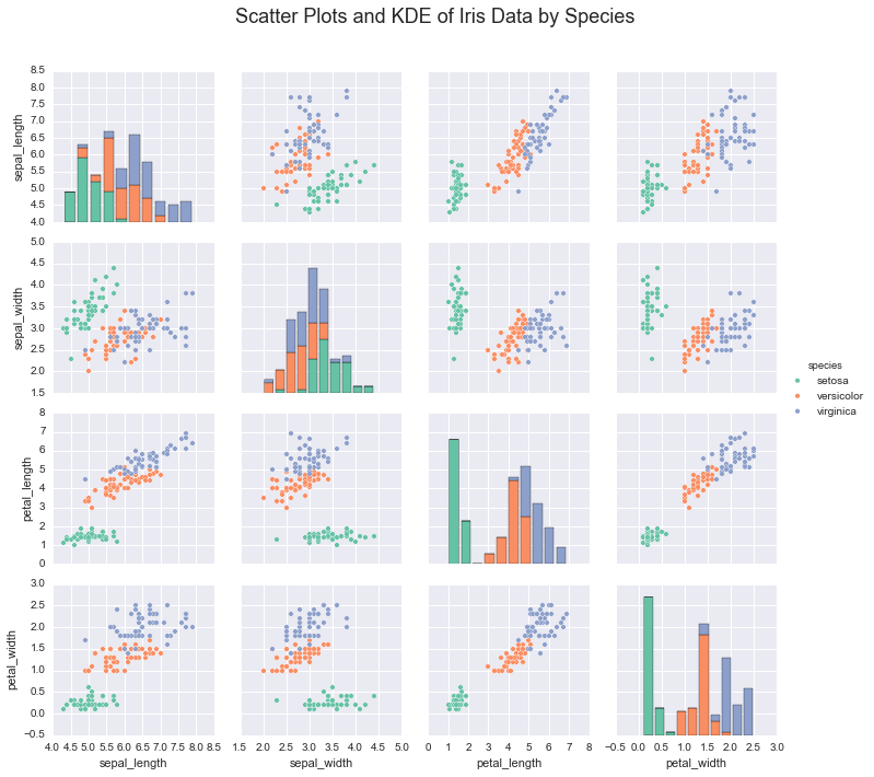
If we wanted to learn these underlying species’ measurements, we would use these real valued measurements and make assumptions about the structure of the data.
For example we could assume that each species had a latent range of mesurements, and assume that these measurements were distributed multivariate normal. In other words, the conditional probability of the measurements given the species would be normally distributed
Bayesian Models allow us to leverage those assumptions.
In the case of the iris dataset, we would be able to learn both the
latent measurements of each Gaussian AND the number of species with a
Dirichlet Process Mixture Model, microscopes.mituremodel
Relational Data
While Dirichlet Process Mixture Models are the most common Bayesian Nonparametric Model, there are other kinds of data to consider. For example, let’s consider relational data in social networks
While social network data also has discrete valued varaibles, in this case they have a different interpretation than the iris dataset
Let’s look at the Enron Email Corpus
import enron_utils


with open('results.p') as fp:
    communications = pickle.load(fp)
def allnames(o):
    for k, v in o:
        yield [k] + list(v)
names = set(it.chain.from_iterable(allnames(communications)))
names = sorted(list(names))
namemap = { name : idx for idx, name in enumerate(names) }
N = len(names)

communications_relation = np.zeros((N, N), dtype=np.bool)
for sender, receivers in communications:
    sender_id = namemap[sender]
    for receiver in receivers:
        receiver_id = namemap[receiver]
        communications_relation[sender_id, receiver_id] = True

print "%d names in the corpus" % N
115 names in the corpus
In this dataset, data is representated as a binary communication matrix where
Let’s visualize the communication matrix
labels = [i if i%20 == 0 else '' for i in xrange(N)]
sns.heatmap(communications_relation, linewidths=0, cbar=False, xticklabels=labels, yticklabels=labels)
plt.xlabel('person number')
plt.ylabel('person number')
plt.title('Email Communication Matrix')
<matplotlib.text.Text at 0x11f764390>
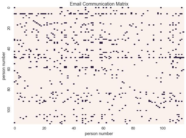
In this context, binary data represents communication between individuals. With this interpretation of the data, we can model the underlying social network.
To learn its structure we could use the Inifinite Relational Model,
microscopes.irm
In the case of time series data, the index of the data describes the relationship between the observation and the rest of the data
For example, let’s look at the Old Faithful Data
old_faithful = pd.read_csv('https://vincentarelbundock.github.io/Rdatasets/csv/datasets/faithful.csv', index_col=0)
old_faithful.head()
| eruptions | waiting | |
|---|---|---|
| 1 | 3.600 | 79 |
| 2 | 1.800 | 54 |
| 3 | 3.333 | 74 |
| 4 | 2.283 | 62 |
| 5 | 4.533 | 85 |
Let’s plot the erruptions as a function of time
f, ax = plt.subplots(figsize=(17, 9))
sns.tsplot(old_faithful['eruptions'], ax=ax)
plt.xlabel('erruptions')
plt.ylabel('time')
<matplotlib.text.Text at 0x120e4fad0>
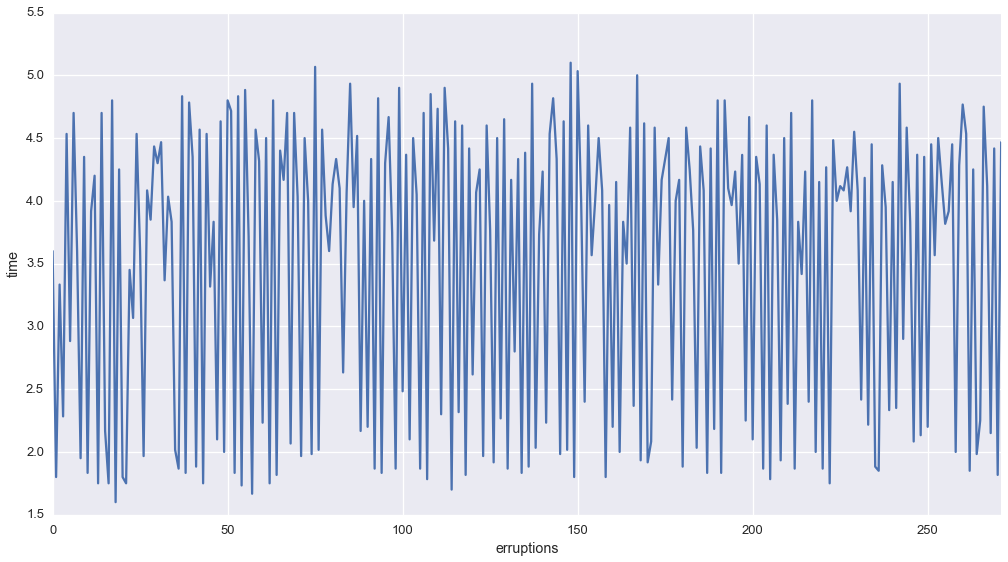
The plot sugests that the number of errupitons has a particular set of states
To learn both the number of underlying states and the states themselves, we could use a Dirichlet-Process Hidden Markov Model
Finally, let’s consider text data
Text data, like social network data, is discrete valued. However, the values are each word or its id.
with open('nyt_50.txt', 'r') as f:
    nyt = f.read()
nyt = nyt.split('\n')
In the case of the New York Times Dataset, we have 50 documents
print nyt[0][:100]
print nyt[1][:100]
the new york times said editorial for tuesday jan new year day has way stealing down upon coming the
the seminal russian filmmaker sergei eisenstein had physically matched the style his monumental film
One of the most common classification tasks within corpora is topic modelling
While LDA is a popular method of topic modeling, we can also learn topics and the number of topics with the Heierarchical Dirichlet Process
These example illustrate the ways in which Bayesian Nonparametric Models can learn structure within data. For more information about each model within Datamicroscopes you can read about each of the models in detail.