Count Data and Ordinal Data with the Gamma-Poisson Distribution¶

Typically, we model count data, or integer valued data, with the gamma-Poisson distribution

Recall that the Poisson distribution is a distribution over integer values parameterized by \(\lambda\). One interpretation behind \(\lambda\) is that it parameterizes the rate at which events occur with a fixed interval, assuming these events occur independently. The gamma distribution is conjugate to the Poisson distribution, so the gamma-Poisson distribution allows us to learn both the distribution over counts and the rate parameter \(\lambda\).

Let’s set up our environment and consider some examples of count data

import pandas as pd
import seaborn as sns
import numpy as np
import matplotlib.pyplot as plt
sns.set_context('talk')
import csv
import urllib2
import StringIO

%matplotlib inline

Children Ever Born is a dataset of birthrates in Fiji from the World Fertility Survey with the following columns:

dur: marriage duration
res: residence,
educ: level of education,
mean: mean number of born,
var: variance of children born
y: number of women

Ordinal columns dur, res, and educ are shown as text in the following dataset

ceb = pd.read_csv('http://data.princeton.edu/wws509/datasets/ceb.dat', sep='\s+')
ceb.head()

	dur	res	educ	mean	var	n	y
1	0-4	Suva	none	0.50	1.14	8	4.00
2	0-4	Suva	lower	1.14	0.73	21	23.94
3	0-4	Suva	upper	0.90	0.67	42	37.80
4	0-4	Suva	sec+	0.73	0.48	51	37.23
5	0-4	urban	none	1.17	1.06	12	14.04

With the these columns encoded, we can now represent them as integers

dur and educ are ordinal columns. Additionally, number of women, n, is integer valued.

ceb_int = pd.read_csv('http://data.princeton.edu/wws509/datasets/ceb.raw', sep='\s+', names = ['index'] + list(ceb.columns[:-1]), index_col=0)
ceb_int.head()

	dur	res	educ	mean	var	n
index
1	1	1	1	0.50	1.14	8
2	1	1	2	1.14	0.73	21
3	1	1	3	0.90	0.67	42
4	1	1	4	0.73	0.48	51
5	1	2	1	1.17	1.06	12

We can map these orderings of dur and educ to produce a crosstab heatmap of n, numbe of women

plt.figure(figsize=(9,6))
ct = pd.crosstab(ceb_int['dur'], ceb_int['educ'], values=ceb_int['n'], aggfunc= np.sum).sort_index(ascending = False)
sns.heatmap(ct, annot = True)
plt.yticks(ceb_int['dur'].drop_duplicates().values - .5, ceb['dur'].drop_duplicates().values)
plt.xticks(ceb_int['educ'].drop_duplicates().values - .5, ceb['educ'].drop_duplicates().values)
plt.ylabel('duration of marriage (years)')
plt.xlabel('level of education')
plt.title('heatmap of marriage duration by level of education')

<matplotlib.text.Text at 0x11a8f48d0>

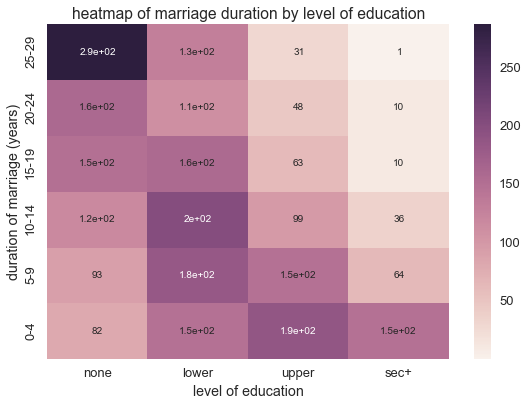
Since dur and education are ordinal valued, the columns assume a small number of integer values

Additionally, the caffeine dataset below measures caffeine intake and performance on a 10 question quiz. The variables are:

coffee: coffee intake (1 = 0 cups, 2 = 2 cups, 3 = 4 cups)
perf: quiz score
numprob: problems attempted
accur: accuracy

response = urllib2.urlopen('http://stanford.edu/class/psych252/_downloads/caffeine.csv')
html = response.read()
caf = pd.read_csv(StringIO.StringIO(html[:-16]))
caf.head()

	coffee	perf	accur	numprob
0	1	53	0.449877	7
1	1	9	0.499534	6
2	1	31	0.498590	6
3	1	38	0.454312	7
4	2	40	0.421212	8

Based on the characteristics of each column, coffee and numprob easily fit into the category of count data appropriate to a gamma-Poisson distribution

caf.describe()

	coffee	perf	accur	numprob
count	60.000000	60.000000	60.000000	60.000000
mean	2.000000	42.366667	0.510854	7.950000
std	0.823387	18.350603	0.107704	1.185005
min	1.000000	5.000000	0.240238	6.000000
25%	1.000000	31.000000	0.425859	7.000000
50%	2.000000	40.000000	0.509806	8.000000
75%	3.000000	53.500000	0.594445	9.000000
max	3.000000	89.000000	0.748692	10.000000

Note that while integer valued data with high values is sometimes modeled with a gamma-Poisson ditribution, remember that the gamma-Poisson distribution has equal mean and variance \(\lambda\):

\[E(X) = Var(X) = \lambda\]

If you want to be more flexible with this assumption, you may want to consider using a normal inverse-chisquare or a normal inverse-Wishart distribution depending on your data

To import the gamma-poisson likelihood, call:

from microscopes.models import gp as gamma_poisson