Binary Data with the Beta Bernouli Distribution¶

Let’s consider one of the most basic types of data - binary data

import pandas as pd
import seaborn as sns
import math
import cPickle as pickle
import itertools as it
import numpy as np
import matplotlib.pyplot as plt
from sklearn.datasets import fetch_mldata
import itertools as it
%matplotlib inline
sns.set_context('talk')

Binary data can take various forms:

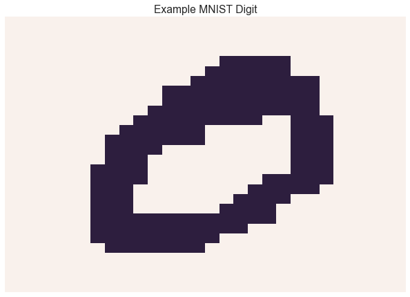
Image data is often represented as binary images. For example, the MNIST dataset contains images of handwritten digits.

Let’s convert the MNIST digits into binary images

mnist_dataset = fetch_mldata('MNIST original')
_, D = mnist_dataset['data'].shape
Y = mnist_dataset['data'].astype(bool)
W = int(math.sqrt(D))
assert W * W == D
sns.heatmap(np.reshape(Y[0], (W, W)), linewidth=0, xticklabels=False, yticklabels=False, cbar=False)
plt.title('Example MNIST Digit')

<matplotlib.text.Text at 0x1127f1910>

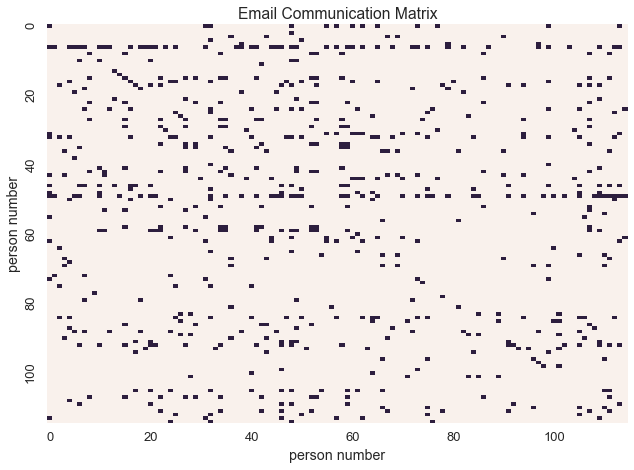
Graphs can be represented as binary matrices

In this email communication network from the enron dataset, \(X_{i,j} = 1\) if and only if person\(_{i}\) sent an email to person\(_{j}\)

import enron_utils


with open('results.p') as fp:
    communications = pickle.load(fp)
def allnames(o):
    for k, v in o:
        yield [k] + list(v)
names = set(it.chain.from_iterable(allnames(communications)))
names = sorted(list(names))
namemap = { name : idx for idx, name in enumerate(names) }
N = len(names)
communications_relation = np.zeros((N, N), dtype=np.bool)
for sender, receivers in communications:
    sender_id = namemap[sender]
    for receiver in receivers:
        receiver_id = namemap[receiver]
        communications_relation[sender_id, receiver_id] = True
labels = [i if i%20 == 0 else '' for i in xrange(N)]
sns.heatmap(communications_relation, linewidths=0, cbar=False, xticklabels=labels, yticklabels=labels)
plt.xlabel('person number')
plt.ylabel('person number')
plt.title('Email Communication Matrix')

<matplotlib.text.Text at 0x11bca0390>

In a Bayesian context, one often models binary data with a beta Bernoulli distribution

The beta Bernoulli distribution is the posterior of the Bernoulli distribution and its conjugate prior the beta distribution

Recall that the Bernouli distribution is the likelihood of \(x\) given some probability \(\theta\)

\[P(x=1)=\theta\]

\[P(x=0)=1-\theta\]

\[P(x|\theta)=\theta^x(1-\theta)^{1-x}\]

If we wanted to learn the underlying probability \(\theta\), we would use the beta distribution, which is the conjugate prior of the Bernouli distribution.

To import our desired distribution we’d call

from microscopes.models import bb as beta_bernoulli

Then given the specific model we’d want we’d import

from microscopes.model_name.definition import model_definition

from microscopes.irm.definition import model_definition as irm_definition
from microscopes.mixture.definition import model_definition as mm_definition

We would then define the model as follows

defn_mixture = mm_definition(Y.shape[0], [beta_bernoulli]*D)
defn_irm = irm_definition([N], [((0, 0), beta_bernoulli)])