Real Valued Data and the Normal Inverse-Wishart Distribution¶

One of the most common forms of data is real valued data

Let’s set up our environment and consider an example dataset

import pandas as pd
import seaborn as sns
import numpy as np
import matplotlib.pyplot as plt
%matplotlib inline
sns.set_context('talk')
sns.set_style('darkgrid')

The Iris Flower Dataset is a standard machine learning data set dating back to the 1930s. It contains measurements from 150 flowers, 50 from each of the following species:

Iris Setosa
Iris Versicolor
Iris Virginica

iris = sns.load_dataset('iris')
iris.head()

	sepal_length	sepal_width	petal_length	petal_width	species
0	5.1	3.5	1.4	0.2	setosa
1	4.9	3.0	1.4	0.2	setosa
2	4.7	3.2	1.3	0.2	setosa
3	4.6	3.1	1.5	0.2	setosa
4	5.0	3.6	1.4	0.2	setosa

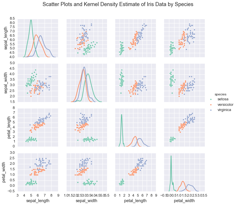
In the case of the iris dataset, plotting the data shows that indiviudal species exhibit a typical range of measurements

irisplot = sns.pairplot(iris, hue="species", palette='Set2', diag_kind="kde", size=2.5)
irisplot.fig.suptitle('Scatter Plots and Kernel Density Estimate of Iris Data by Species', fontsize = 18)
irisplot.fig.subplots_adjust(top=.9)

If we wanted to learn these underlying species’ measurements, we would use these real valued measurements and make assumptions about the structure of the data.

In practice, real valued data is commonly assumed to be distributed normally, or Gaussian

We could assume that conditioned on species, the measurement data follwed a multivariate normal

\[P(\mathbf{x}|species=s)\sim\mathcal{N}(\mu_{s},\Sigma_{s})\]

The normal inverse-Wishart distribution allows us to learn the underlying parameters of each normal distribution, its mean \(\mu_s\) and its covariance \(\Sigma_s\). Since the normal inverse-Wishart is the conjugate prior of the multivariate normal, the posterior distribution of a multivariate normal with a normal inverse-Wishart prior also follows a normal inverse-Wishart distribution. This allows us to infer the distirbution over values of \(\mu_s\) and \(\Sigma_{s}\) when we define our model.

Note that if we have only one real valued variable, the normal inverse-Wishart distribution is often referred to as the normal inverse-gamma distribution. In this case, we learn the scalar valued mean \(\mu\) and variance \(\sigma^2\) for each inferred cluster.

Univariate real data, however, should be modeled with our normal invese-chi-squared distribution, which is optimized for infering univariate parameters.

See Murphy 2007 for derrivations of our normal likelihood models

To specify the joint distribution of a multivariate normal inverse-Wishart distribution, we would import our likelihood model

from microscopes.models import niw as normal_inverse_wishart