Finding the number of clusters with the Dirichlet Process¶

The Iris Flower Dataset is a standard machine learning data set dating back to the 1930s. It contains measurements from 150 flowers.

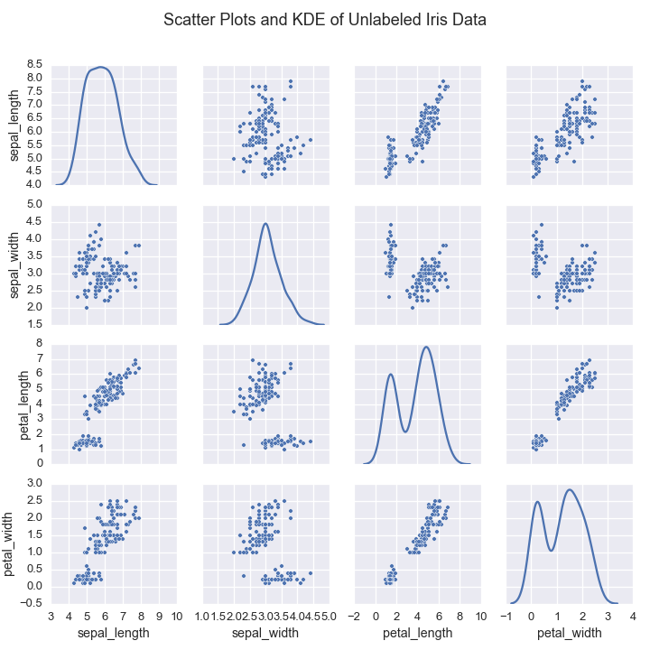
If we wanted to learn these underlying species’ measurements, we would use these real valued measurements and make assumptions about the structure of the data. We could assume that conditioned on assignment to species, the measurement data follwed a multivariate normal

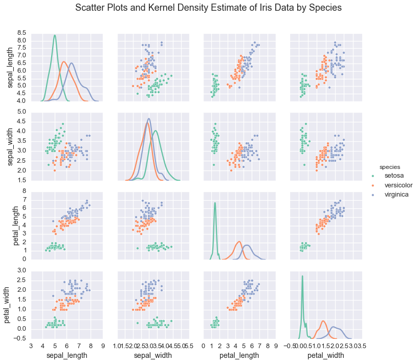
In this case, the data comes from three species of flowers:

• Iris Setosa
• Iris Versicolor
• Iris Virginica

Plotting the data shows that indiviudal species exhibit a typical range of measurements

The dimensionality of a clustering model is equal to the number of clusters in the model. Bayesian clustering algorithms often rely of the Dirichlet Distribution to encode prior information about these cluster assignments. The Dirichlet distribution (DD) can be considered a distribution of distributions. Each sample from the DD is a categorial distribution over \(K\) categories. It is parameterized \(G_0\), a distribution over \(K\) categories and \(\alpha\), a scale factor.

The expected value of the DD is \(G_0\). The variance of the DD is a function of the scale factor. When \(\alpha\) is large, samples from \(DD(\alpha\cdot G_0)\) will be very close to \(G_0\). When \(\alpha\) is small, samples will vary more widely.

Most clustering algorithms require the number of clusters to be given in advance. If we don’t know the number of species in the data, how would we be able to classify these flowers?

The Dirichlet Process is a stochastic process used in Bayesian nonparametrics to cluster data without specifying the number of clusters in advance. The Dirichlet Process Prior is used to mathematically descirbe prior information about the number of clusters in the data.

The Dirichlet Process Prior is nonparametric because its dimensionality is infinite. This characteristic is advantageous in clustering because it allows us to recognize new clusters when we observe new data.

The Dirichlet Process can be considered a way to generalize the Dirichlet distribution. While the Dirichlet distribution is parameterized by a discrete distribution \(G_0\) and generates samples that are similar discrete distributions, the Dirichlet process is parameterized by a generic distribution \(H_0\) and generates samples which are distributions similar to \(H_0\). The Dirichlet process also has a parameter \(\alpha\) that determines how similar how widely samples will vary from \(H_0\).

When learning a clustering using a Dirichlet Process Prior, observations are probabilistically assigned to clusters based on the number of observations in that cluster \(n_k\).

Probability of new clusters are paramteterized by \(\alpha\)

In other words, these culsters exhbit a rich get richer property.

The expected number of clusters in a dataset clustered with the Dirichlet Process is \(O(\alpha\log(N))\)

The expected number of clusters with \(m\) observations (Arratia et al., 2003) is \(\frac{\alpha}{m}\)

We can construct a sample \(H\) (recall that \(H\) is a probability distribution) from a Dirichlet process \(\text{DP}(\alpha H_0)\) by drawing a countably infinite number of samples \(\theta_k\) from \(H_0\)) and setting:

where the \(\pi_k\) are carefully chosen weights (more later) that sum to 1. (\(\delta\) is the Dirac delta function.)

\(H\), a sample from \(DP(\alpha H_0)\), is a probability distribution that looks similar to \(H_0\) (also a distribution). In particular, \(H\) is a discrete distribution that takes the value \(\theta_k\) with probability \(\pi_k\). This sampled distribution \(H\) is a discrete distribution even if \(H_0\) has continuous support; the support of \(H\) is a countably infinite subset of the support \(H_0\).

The weights (\(\pi_k\) values) of a Dirichlet process sample related the Dirichlet process back to the Dirichlet distribution.

Gregor Heinrich writes:

The defining property of the DP is that its samples have weights \(\pi_k\) and locations \(\theta_k\) distributed in such a way that when partitioning \(S(H)\) into finitely many arbitrary disjoint subsets \(S_1, \ldots, S_j\) \(J<\infty\), the sums of the weights \(\pi_k\) in each of these \(J\) subsets are distributed according to a Dirichlet distribution that is parameterized by \(\alpha\) and a discrete base distribution (like \(G_0\)) whose weights are equal to the integrals of the base distribution \(H_0\) over the subsets \(S_n\).

As an example, Heinrich imagines a DP with a standard normal base measure \(H_0\sim \mathcal{N}(0,1)\). Let \(H\) be a sample from \(DP(H_0)\) and partition the real line (the support of a normal distribution) as \(S_1=(-\infty, -1]\), \(S_2=(-1, 1]\), and \(S_3=(1, \infty]\) then

where \(H(S_n)\) be the sum of the \(\pi_k\) values whose \(\theta_k\) lie in \(S_n\).

These \(S_n\) subsets are chosen for convenience, however similar results would hold for any choice of \(S_n\). For any sample from a Dirichlet process, we can construct a sample from a Dirichlet distribution by partitioning the support of the sample into a finite number of bins.

There are several equivalent ways to choose the \(\pi_k\) so that this property is satisfied: the Chinese restaurant process, the stick-breaking process, and the Pólya urn scheme.

To generate \(\left\{\pi_k\right\}\) according to a stick-breaking process we define \(\beta_k\) to be a sample from \(\text{Beta}(1,\alpha)\). \(\pi_1\) is equal to \(\beta_1\). Successive values are defined recursively as

Thus, if we want to draw a sample from a Dirichlet process, we could, in theory, sample an infinite number of \(\theta_k\) values from the base distribution \(H_0\), an infinite number of \(\beta_k\) values from the Beta distribution. Of course, sampling an infinite number of values is easier in theory than in practice.

However, by noting that the \(\pi_k\) values are positive values summing to 1, we note that, in expectation, they must get increasingly small as \(k\rightarrow\infty\). Thus, we can reasonably approximate a sample \(H\sim DP(\alpha H_0)\) by drawing enough samples such that \(\sum_{k=1}^K \pi_k\approx 1\).

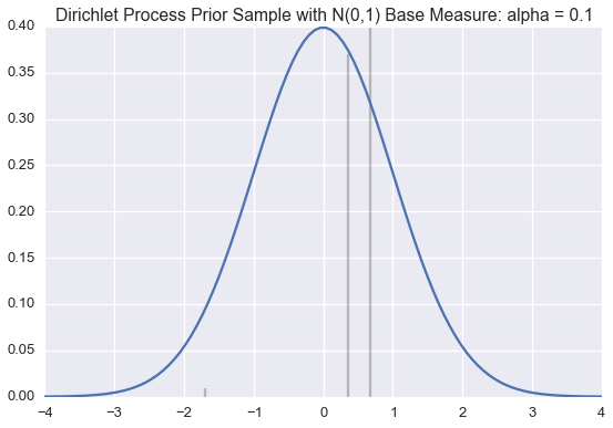
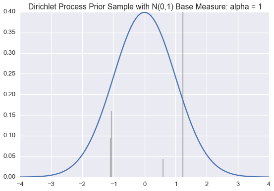
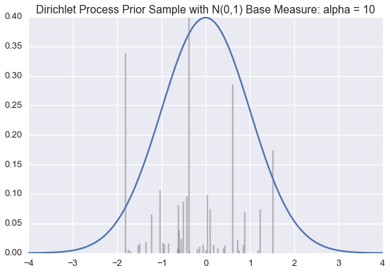
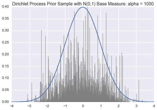
We use this method below to draw approximate samples from several Dirichlet processes with a standard normal (\(\mathcal{N}(0,1)\)) base distribution but varying \(\alpha\) values.

Recall that a single sample from a Dirichlet process is a probability distribution over a countably infinite subset of the support of the base measure.

The blue line is the PDF for a standard normal. The black lines represent the \(\theta_k\) and \(\pi_k\) values; \(\theta_k\) is indicated by the position of the black line on the \(x\)-axis; \(\pi_k\) is proportional to the height of each line.

We generate enough \(\pi_k\) values are generated so their sum is greater than 0.99. When \(\alpha\) is small, very few \(\theta_k\)‘s will have corresponding \(\pi_k\) values larger than \(0.01\). However, as \(\alpha\) grows large, the sample becomes a more accurate (though still discrete) approximation of \(\mathcal{N}(0,1)\).

Often we want to draw samples from a distribution sampled from a Dirichlet Process instead of from the Dirichlet process itself. Much of the literature on the topic unhelpful refers to this as sampling from a Dirichlet process.

Fortunately, we don’t have to draw an infinite number of samples from the base distribution and stick breaking process to do this. Instead, we can draw these samples as they are needed.

Suppose, for example, we know a finite number of the \(\theta_k\) and \(\pi_k\) values for a sample \(H\sim \text{Dir}(\alpha H_0)\). For example, we know

To sample from \(H\), we can generate a uniform random \(u\) number between 0 and 1. If \(u\) is less than 0.5, our sample is \(0.1\). If \(0.5<=u<0.8\), our sample is \(-0.5\). If \(u>=0.8\), our sample (from \(H\) will be a new sample \(\theta_3\) from \(H_0\). At the same time, we should also sample and store \(\pi_3\). When we draw our next sample, we will again draw \(u\sim\text{Uniform}(0,1)\) but will compare against \(\pi_1, \pi_2\), AND \(\pi_3\).

The class below will take a base distribution \(H_0\) and \(\alpha\) as arguments to its constructor. The class instance can then be called to generate samples from \(H\sim \text{DP}(\alpha H_0)\).

from numpy.random import choice

class DirichletProcessSample():
    def __init__(self, base_measure, alpha):
        self.base_measure = base_measure
        self.alpha = alpha

        self.cache = []
        self.weights = []
        self.total_stick_used = 0.

    def __call__(self):
        remaining = 1.0 - self.total_stick_used
        i = DirichletProcessSample.roll_die(self.weights + [remaining])
        if i is not None and i < len(self.weights) :
            return self.cache[i]
        else:
            stick_piece = beta(1, self.alpha).rvs() * remaining
            self.total_stick_used += stick_piece
            self.weights.append(stick_piece)
            new_value = self.base_measure()
            self.cache.append(new_value)
            return new_value

    @staticmethod
    def roll_die(weights):
        if weights:
            return choice(range(len(weights)), p=weights)
        else:
            return None

This Dirichlet process class could be called stochastic memoization. This idea was first articulated in somewhat abstruse terms by Daniel Roy, et al.

Below are histograms of 10000 samples drawn from samples drawn from Dirichlet processes with standard normal base distribution and varying \(\alpha\) values.

import pandas as pd

base_measure = lambda: norm().rvs()
n_samples = 10000
samples = {}
for alpha in [1, 10, 100, 1000]:
    dirichlet_norm = DirichletProcessSample(base_measure=base_measure, alpha=alpha)
    plt.figure(figsize=(9,6))
    pd.Series([dirichlet_norm() for _ in range(n_samples)]).hist()
    plt.title('Alpha: %s' % alpha)
    plt.savefig('Alpha_Hist_%s.png')

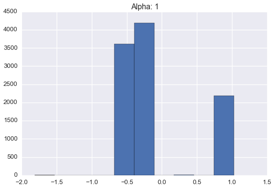
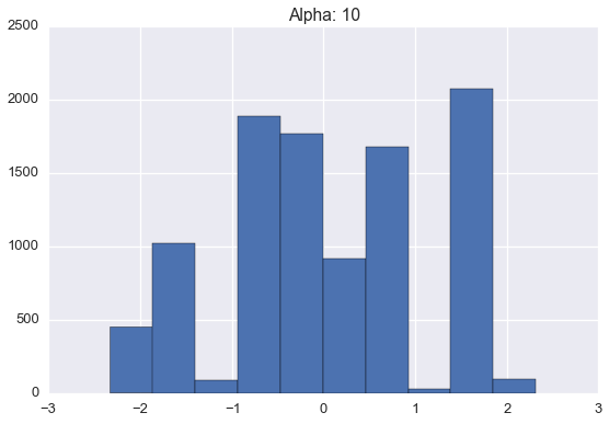
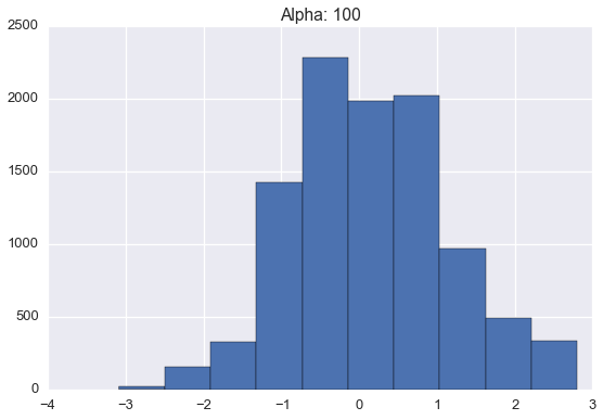
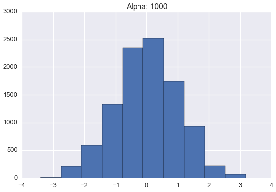
Note that these histograms look very similar to the corresponding plots of sampled distributions above. However, these histograms are plotting points sampled from a distribution sampled from a Dirichlet process while the plots above were showing approximate distributions samples from the Dirichlet process. Of course, as the number of samples from each \(H\) grows large, we would expect the histogram to be a very good empirical approximation of \(H\).

For more information on the Dirichlet Process, please see our developer Tim Hopper’s additional notebooks.